Different Functions in Google Sheets

Hi everybody I’m Dylan and I hope that you are doing well. Today I am going to be showing you 3 different functions that you can use in Google Sheets. In my previous blog post I talked about the SUM functions so if you are looking for that check out my previous blog post “Adding Numbers in Google Sheets. Also if you want to see this blog post in video form be sure to check out my YouTube Channel “Dylan Excel or the video link at the bottom of this page.

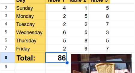
Function 1: COUNT

For the first function I’m going to be talking about COUNT, it is a similar function to SUM, but instead of counting all of the numbers in the cell it will count all of the cells individually. To use this function we must first find the area in the spreadsheet, for example E4 to G9. Next we need to plug our count formula into the formula tab. This is the usually empty row that can be found by the “fx” on the far right of it, now we need to type in the formula.

First type a = sign in the formula bar, next follow it with the function, in this case its “COUNT”, now you can type where your information is, and in my case like I said before mine is from E4 to G9, but this will change for you. So in the end my equation should look like “=COUNT(E4:G9)” make sure you have the cell you want your equation in then you should be able to click off of your cell or click “Enter” on your keyboard to process the equation.

Function 2: AVERAGE

For the second function, I’m going to be talking about AVERAGE. This function is great when you want to find the average value of a range of numbers in your spreadsheet. Instead of adding up all the numbers yourself and then dividing by the total count, AVERAGE does all of that for you automatically.

Calculate an average in Google Sheet

To use the AVERAGE function, start by clicking on the cell where you want the average to appear. Then, just like with the COUNT function, go to the formula bar (the one by the ‘fx’ symbol). Type of course the = sign followed by AVEREAGE and then input the range of cells you want to average. For example, if you want to find the average of the numbers in cells B2 through B10, you would type =AVERAGE(B2:B10)

Function 3: MIN & MAX

For the final function I wanted to talk about the MIN & MAX functions, these two are technically different functions but they are so similar that they work together while explaining or using them. First, let’s start with the MAX function. This function helps you find the largest number in a range of cells.

Use Min and Max in Google Sheets

To use it, just like before, select the cell where you want the result to appear, then go to the formula bar. Following the same way we have done this before type in the = sign then put in the MAX function, then input the range of cells you’re analyzing. For example, if you want to find the maximum value between cells C3 and C12, your formula would look like this: =MAX(C3:C12) after that you can click off the cell or click the enter button to process the equation.

Video: “Using Functions in Google Sheets!”

About the Author

Dylan S is a 4th year Design Studio student, at a high school in Toronto, Canada. As the summer intern at Contextures, Dylan is adding spreadsheet and video skills to his repertoire. We’re excited to see him share those new skills online, through his videos and articles.